Economic rent of land as a fraction of Australian GDP

Gavin R. Putland updates Terry Dwyer's “The Taxable Capacity of Australian Land and Resources”.

The normal return on capital — meaning produced capital — is needed to motivate its formation and is therefore part of the cost of its product. Hence a tax on produced capital, no less than a tax on labour, suppresses production and raises prices. That is why the precise implementation of “fiscal devaluation” — a uniform cut in production costs through tax reform — requires cutting taxes on both labour and capital (Putland, 2013). But land is different. As land is a gift of nature, its total return (comprising current rent and “capital gains”) is not a cost of production, but a surplus (“economic rent”), which may be appropriated for public revenue without impeding production or raising prices.

(The term “capital gain” will be kept in quotation marks because it is a misnomer. In the present context, the gain is in the price of land, not the price of capital. In general, at least in the long term, “real capital doesn't gain”; if appreciation of produced capital were to continue for any considerable time, this would induce the production of more capital until competition reduced its value to a level commensurate with production costs and depreciation. Any assets for which this mechanism does not operate must be land-like in the sense that they cannot be freely reproduced by competitors.)

That a particular piece of land has been rented or bought or mortgaged has implications concerning who receives or has received the surplus, but does not eliminate the surplus. For example, if you own and operate retail premises in a high-traffic location, some of your “value added” is rent of location. If the premises are heavily mortgaged, the rent still exists, but most of it flows to parties other than you.

Neither was the surplus diminished by industrialization and the attendant urbanization. On the contrary, because land is a finite resource, and because access to land is essential to economic participation, the price of access tends to absorb capacity to pay, even as new industries add to that capacity. As Adam Smith (1789, V.2.74) observed,

A tax upon ground-rents would not raise the rents of houses. It would fall altogether upon the owner of the ground-rent, who acts always as a monopolist, and exacts the greatest rent which can be got for the use of his ground. More or less can be got for it according as the competitors happen to be richer or poorer, or can afford to gratify their fancy for a particular spot of ground at a greater or smaller expence. In every country the greatest number of rich competitors is in the capital, and it is there accordingly that the highest ground-rents are always to be found.

Indeed, the persistence of housing stress in the teeth of rising “real” wages and falling “real” construction costs would be inexplicable if the difference were not absorbed by rising ground-rents. The unaffordable ingredient of housing is not the houses themselves, but the space that they occupy and enclose.

All this was well understood by Henry George (1879, III.II.11), who popularized the idea that the rent of land was the proper source of public revenue.

Mainstream economists reacted, in part, by playing down the size of the rent fund. Industrialization and urbanization became excuses to claim that land values were of declining importance, as if houses and factories and commercial buildings did not occupy land, or as if the growth of secondary industries did not increase the capacity to pay for such occupation. Ely (1927, p.131) laid it down as a “formal definition” that “with increasing wealth and stationary population, land values will decline” (Ely's italics; quoted in Gaffney, 1994, Pt.3, p.68). Even Scott (1986, p.38), to whom the present work is heavily indebted, remarked that “A declining share for the value of land in the national wealth is to be expected from a growth of other assets” (quoted by Dwyer, 2003, pp. 29–30). Heilbroner (1980, p.187) was dismissive: “Suffice it to point out that rental income in the United States has shrunk from 6 percent of the national income in 1929 to less than 2 percent today.” Authors of more recent undergraduate texts, such as Case & Fair (1994, p.559), Krugman & Wells (2006, p.283) and Buchholz (2007, p.86), have claimed that rent in the USA is one percent of GDP or less.

If the last claim were true, it would not be a valid argument against collecting as much rent as possible, in order to minimize taxation of labour and capital. But the claim lacks credibility. If there are 125 million homes in the USA (Kendall, 2008), with an average value of $250,000, of which 50% is land value, then the total value of residential land alone is more than $15 trillion, or about a year's GDP. [A 50% land-value fraction is conservative because about half the buildings are more than 35 years old (Kendall, 2008) and therefore contribute little to the resale value, while the rest are in various stages of depreciation.] So, if 70% of the total land value is residential, the total land value is about 1.4 years' GDP. At a rental yield of 5% per annum, the current rent would be 7% of GDP. That does not include “capital gains”. Neither does it account for other “land-like” assets.

Owner-occupancy of land does not reduce the rent or make it less real. To the extent that the land is rented, the rental value accrues to (or through) the landlords. To the extent that the land is owner-occupied, the value does not vanish or shrink just because the owner and the occupant are the same; if it did, nobody would want to be an owner-occupant. Specifically, the rental value accrues to (or through) the owner-occupants in their capacity as owners.

Australian data

The above “back-of-envelope” calculation for the USA is obviously rough. For Australia we can do considerably better. The following graph shows how the estimated economic rent of land, as a fraction of Australian GDP (left-hand scale), has varied over the last century. The “year” means the “financial year ended”. The blue band, including the magenta segments, shows the rental value assuming a yield of 5% per annum. The green band shows the real “capital gains” assuming that 6% of the land value is sold each year, having been bought 8 years earlier; hence no “capital gains” are shown for the first 8 years. Where green gives way to magenta (1919–22, 1938–49), the “capital gains” are negative, so the rental value is indicated by the top of the magenta band (on the left-hand scale). The red band shows tax for all levels of government as a fraction of GDP (inverted right-hand scale). The orange band — the meat in the sandwich — shows what is left for labour and “capital”.

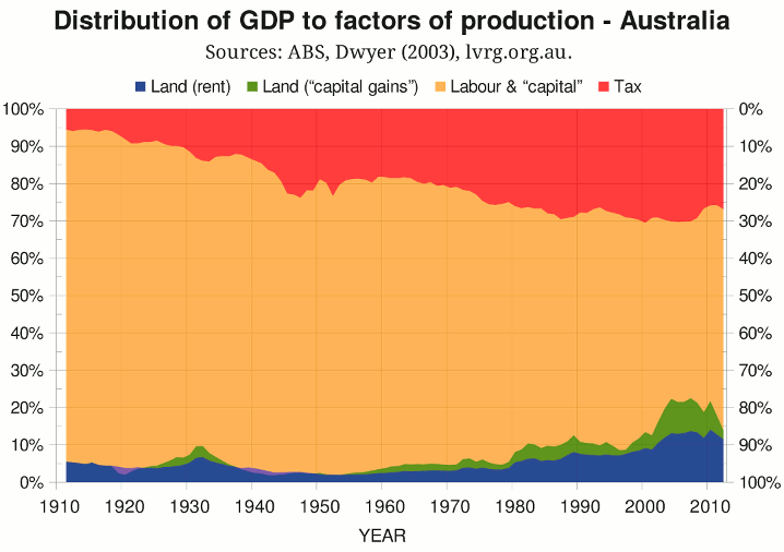
Sources for the graph are as follows:

• The “land value” is the total price of residential, commercial and rural land. Values for 1989 onward are from the Australian Bureau of Statistics (ABS 5204.0, Table 61). Earlier values were compiled by Dwyer (2003, Table 4), citing Scott (1969, 1986) and Herps (1985, 1988). Dwyer's figures for 1980–83 rely on proportionalities between urban and rural values and (less importantly) between the total for the six States and the total for the Territories. His figures for 1984–88 are from ABS 5241.0, 1995, Table 3.2 (p.31).

• The Reserve Bank of Australia has plotted Australia's “dwelling turnover rate” — that is, the ratio of annualized dwelling turnover to estimated dwelling stock — for 1995 through 2010 (RBA, 2011, Graph 3.6). A turnover rate of 6% per annum is typical of that period. For want of further data, and in order to smooth out the realization (cashing in) of “capital gains” on land, I assume that 6% of the land value is sold per year. I further assume, for want of more detailed data, that the land sold each year has been held for 8 years — this period being slightly shorter than the average for dwellings sold in 2012, but slightly longer than the average for dwelling sold in 2002 (RP Data, 2013).

• For the purpose of calculating real “capital gains”, the cost base is adjusted in proportion to an ABS CPI sequence obtained by splicing the “CPI - long-term price series” up to 2000 (ABS 1301.0, 2002) with the standard CPI series for the June quarter (ABS 6401.0, Tables 1&2, series ID A2325846C).

• From 1960 onward, the total tax and total GDP are from ABS 5206.0, Table 18 (series ID A2301963V) and Table 1 (series ID A2302467A). Up to 1959, the total tax and the tax/GDP ratio are from Dwyer (2003), citing Vamplew (1987, Table GF1-7, p.256) and RBA (1996, Table 2.8). Dividing the total tax by the tax/GDP ratio yields an “implied GDP”. For total tax, the Dwyer and ABS figures overlap from 1960 to 1999, and the discrepancies are within ±5%. Dwyer's implied GDP and the ABS's GDP overlap from 1960 to 1995, and the ABS figures are consistently higher, the biggest discrepancy being 16% for 1960. For want of better information, I have attributed the higher values of newer GDP figures to improved methodology, and scaled up the “implied GDP” figures so that they match the ABS figures at 1960. This decision seems to be vindicated by the graph, which shows no discontinuity in the tax share of GDP between 1959 and 1960 (that is, between 1959.5 and 1960.5 on the horizontal axis); if the “implied GDP” had not been scaled up, the tax share prior to 1960 would be higher by about 16% (not to be confused with 16 percentage points).

Paper gains

The second graph (below) shows what happens if the realized “capital gains” are replaced by the smoothed total “paper gain” — that is, the increase in the real total land price over the last year, assuming exponential growth over the last eighteen years (for example, the “paper gain” for 2008 is calculated on the real total land value in 1990 and 2008).

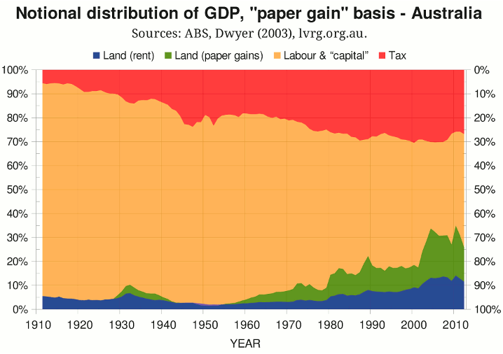
The resulting distribution of GDP is only “notional” because the “paper gains” were not, and could not have been, simultaneously realized. Any attempt to realize them all by selling the land would have caused prices to plummet. Any attempt to realize them all by borrowing against them would have either raised interest rates (reducing the ability to spend the borrowings) or expanded the money supply (eroding purchasing power). Gains that cannot be realized cannot be used as public revenue. Thus, for the purposes of assessing the share of GDP flowing to land and the potential of land to yield public revenue, the first graph is more relevant than the second.

The exclusion of unrealized “capital gains” is a departure from the methodology of Dwyer, as cited by Kavanagh (2007, Fig.1, p.6). Dwyer's approach does not consider realization, but attempts to “level out a growing annuity” (2003, p.55). If the resulting “level” annuity were the sole source of public revenue, it would prevent real revenue from growing with real GDP — to the delight of libertarians, undoubtedly, but in defiance of history.

Returns to labour and capital

The third graph shows the same information as the first, except that the bands for rent and “capital gains” are inverted and stacked with the tax band.

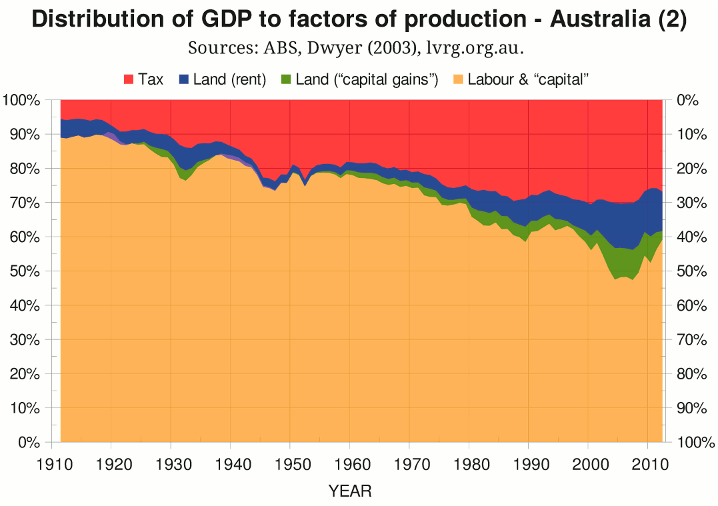
It can be seen that in the four years preceding the “Global Financial Crisis”, the share of GDP accruing to labour and “capital” (left-hand scale) was less than half. The recession of the early '90s followed another notable squeeze on labour and “capital”.

In the graph, “capital” is in quotation marks because it wrongly includes land-like assets other than terra firma. [This is done for want of data on the historical values of such assets; but current values are taken into account by Fitzgerald (2013).] The excessively wide scope of “capital” tends to overstate the share of GDP accruing to the active factors of production (labour and capital). This tendency is partly offset by failing to allow for the incidental capture of land rents and “capital gains” through the income-tax system, which cuts into the share of GDP taken by land. But the degree of “incidental capture” is less than would be suggested by nominal rates of income tax. Imputed rents are not explicitly assessed and are captured only to the extent that they are realized or disguised as assessable income. “Capital gains” on owner-occupied residential land, and on all assets acquired before 1985, are exempt, while “capital gains” on assets acquired by individuals after 1985 have always received concessional treatment (5-year averaging before 1999 and discounting thereafter).

ATCOR/EBCOR

If the price of access to land absorbs capacity to pay, any reduction in that capacity due to taxation is a reduction in the price of access to land. As John Locke (1691) explained,

It is in vain in a country whose great fund is land to hope to lay the publick charge of the Government on anything else; there at last it will terminate. The merchant (do what you can) will not bear it, the labourer cannot, and therefore the landholder must: and whether he were best to do it by laying it directly where it will at last settle, or by letting it come to him by the sinking of his rents,... let him consider.

He went on to assert that even where the great fund appeared to be trade, as in Holland, taxes on trade were borne by landowners.

This reasoning applies not only to the tax payments themselves, but also to the excess burden (or deadweight cost) — that is, the suppression of production as taxes cause otherwise viable ventures to become unviable. As Gaffney (2009) puts it, “All Taxes Come Out of Rents” (ATCOR), and “Excess Burdens Come Out of Rents” (EBCOR).

Under the EBCOR heading we might include the suppression of public investment in infrastructure, due to the failure of the tax system to capture uplifts in land values. The benefit of infrastructure, net of user charges (fees, fares, tolls), is shown in prices of access to locations where that benefit is available — in other words, land values. If the responsible government, through the tax system, receives a certain fraction of every uplift in land value, infrastructure projects whose cost/benefit ratios are less than that fraction are profitable for the government and will therefore proceed. They are profitable because they expand the revenue base without any increase in tax rates. But if the government fails to capture uplifts in land values, some infrastructure projects do not proceed, so that the associated uplifts in land values do not occur, while other projects proceed at the cost of unnecessarily high tax rates and ensuing deadweight costs.

By itself, the ATCOR principle would imply that if existing taxes were abolished, the resulting increase in the economic rent of land would be just enough to replace the forgone revenue,* in which case, if the forgone revenue were indeed replaced by a charge on land, the remainder of the economic rent of land (hence its capitalized price) would be as before. Together, the ATCOR and EBCOR principles would imply that if existing taxes were abolished, the resulting increase in the economic rent of land would be more than enough to replace the forgone revenue, in which case, if the forgone revenue were indeed replaced by a charge on land, the remainder of the economic rent of land (hence its capitalized price) would be more than before.

The same conclusions can be reached by considering locational arbitrage. Suppose you wish to rent or buy a site. Suppose you have a choice between two adjacent sites, equally desirable in every way except that they happen to be on opposite sides of the border between two jurisdictions. In one jurisdiction, you must pay $x/year in “tax” on the site. In the other, you must pay $x/year in tax on the proceeds of your intended use of the site. Would you offer less for the site in the former jurisdiction just because the “tax” is on the site itself? Would you not rather offer more in order to avoid the cost, risk and inconvenience of self-assessing your tax liability? What if the competing sites were further from the border, so that the earning opportunities attached to the sites were affected by the deadweight costs of the tax systems in their respective jurisdictions? Would you not be willing to offer more for the site on which the earning opportunities were not diminished by deadweight?

The same conclusions can be reached by considering the net present value (NPV) of an investment. If you are going to rent a site for a number of years, or buy it and resell it after the same number of years, any taxes and tax-related costs that you must incur over that period are a deduction (in NPV terms) from the rent or purchase price that you could otherwise justify paying over the same period. The same logic applies to other prospective bidders for the site. It is immaterial whether the “tax” is payable on the rental value of the land, or on the “capital gain”, or on some specified proceeds of the actual use of the land: the more the market must pay under the guise of tax, the less it will pay as rent, or as interest on the purchase price of the future rent stream.

So, if any increase in public revenue from land is used to reduce taxes on other bases, it should not reduce rents or prices that people are willing to pay for land. And those rents and prices tend to grow as the economy grows.

Mechanisms that counteract ABCOR/EBCOR

If reductions in taxes and deadweight costs incurred by tenants were competed away in higher rents, there would be no improvement in affordability of accommodation. But the tax benefits would not be entirely competed away, because public charges on land values relieve artificial shortages caused by speculation. A sufficiently high holding charge makes it uneconomic to hold vacant lots or unoccupied buildings. The resulting need to generate income from landed property, or to let it or sell it to someone who will, strengthens the bargaining positions of tenants and buyers relative to landlords and sellers. A charge on “capital gains”, by default, makes it more necessary to generate current income from property, improving the bargaining positions of tenants. Thus the financing of government from charges on land values enhances equity (helping the less wealthy), but not at the expense of efficiency (maximizing production).

Significance of current rents

The ATCOR principle says that if existing taxes were abolished, the resulting increase in the economic rent of land would be enough to replace the forgone revenue, without tapping into existing returns on land. For the purpose of replacing existing taxes with land-based revenue, the existing economic rent of land is the margin for error in the ATCOR principle. That margin is needed in case the downward effect on rents due to the stronger bargaining positions of tenants and buyers outweighs the upward effect on rents due to the EBCOR mechanism.

Conclusion

In Australia in 2011-12, taxes amounted to about 27% of GDP, while the economic rent of land (current rents and smoothed “capital gains”) amounted to about 14% of GDP. The theory that all taxes come out of rents (ATCOR), suggests that if the taxes were abolished, the economic rent of land would rise by 27% of GDP. But even if the ATCOR effect were overestimated by a factor of two, so that the economic rent of land rose by only 13.5% of GDP, the resulting economic rent would still be enough to replace existing taxes.

References

__________

* Whether the present economic rents from all sources, depleted as they are by present taxes and their deadweight costs, would be enough to replace the revenue from those taxes is a different question, and is examined by Fitzgerald (2013).

[Last modified 11 July 2013.]

References

Buchholz, T.G., New Ideas from Dead Economists (Plume, 2007).
Case, K.E. & Fair, R.C., Economics, 3rd Ed. (Prentice-Hall, 1994).
Dwyer, T.M., “The Taxable Capacity of Australian Land and Resources”, Australian Tax Forum, vol.18 (2003), pp. 21–68.
Ely, R.T., 1927, “Land Economics”, in Hollander, J. (ed.), Economic Essays Contributed in Honor of John Bates Clark (New York: Macmillan, 1927), pp. 119–35. Reprinted Freeport, NY: Books for Libraries Press, 1967. Quoted by Gaffney (1994, q.v.).
Fitzgerald, K.B., 2013 (upcoming), Total Resource Rents of Australia (Melbourne: Prosper Australia).
Gaffney, M., 1994, “Neo-classical Economics as a Stratagem against Henry George”, in Gaffney, M., Harrison, F., and Feder, K., The Corruption of Economics (London: Shepheard-Walwyn, 1994), pp. 29–164. Online: is.gd/gaffney1994.
Gaffney, M., 2009, “The hidden taxable capacity of land: enough and to spare”, International Journal of Social Economics, vol.36, no.4 (2009), pp. 328–411.
George, H., 1879, Progress and Poverty. Reprinted Garden City, NY: Doubleday, Page & Co., 1920. Online: is.gd/George1879 (Library of Economics and Liberty).
Heilbroner, R.L., The Worldly Philosophers, 5th Ed. (New York: Simon & Schuster, 1980).
Herps, M.D., 1985 Review of Tax Relativities: Relative Capacities of States and the Northern Territory to Raise Land Revenues (Canberra: Commonwealth Grants Commission, 1985). Cited by Dwyer (2003, q.v.) and Soos (2013, q.v.).
Herps, M.D., 1988, “Review of General Revenue Grant Relativities: Relative Capacities of States and Northern Territory to Raise Land Revenues”, in Commonwealth Grants Commission, Report on General Revenue Grant Relativities 1988, Volume II (Canberra, 1988). Cited by Dwyer (2003, q.v.) and Soos (2013, q.v.).
Kavanagh, B.L., Unlocking the Riches of Oz (Melbourne: Land Values Research Group, 2007). Online: lvrg.org.au/files/riches-of-oz.pdf.
Kendall, C., “How many houses are there in the US?” Understanding the Market, 24 June 2008. Online: understandingthemarket.com/?p=15.
Krugman, P.R. & Wells, R., Economics (Worth Publishers, 2006). Quoted in Fitzgerald (2013, q.v.).
Locke, J., Some considerations of the consequences of the lowering of interest, and raising the value of money (attached to a letter to Sir John Somers MP, 7 Nov. 1691). Online: is.gd/locke1691 (Hamilton, ON: McMaster University).
Putland, G.R., “Misrepresentation of ‘fiscal devaluation’ in the Weekend Australian”, 7 July 2013. Online: is.gd/mofdio.
RBA, 1996, Australian Economic Statistics 1949–50 to 1994–95 (Sydney: Reserve Bank of Australia, 1996). Cited by Dwyer (2003, q.v.).
RBA, 2011, Statement on Monetary Policy, August 2011 (Sydney: Reserve Bank of Australia). Online: is.gd/rbasmp201108.
RP Data, Home owners staying put! (National Media Release, 7 March 2013).
Scott, R.H., 1969, The Value of Land in Australia (Sydney: Reserve Bank of Australia, 1969). Cited by Dwyer (2003, q.v.) and Soos (2013, q.v.).
Scott, R.H., 1986, The Value of Land in Australia (Canberra: Centre for Research on Federal Financial Relations, Australian National University, 1986). Cited by Dwyer (2003, q.v.) and Soos (2013, q.v.).
Smith, A., 1789, An Inquiry into the Nature and Causes of the Wealth of Nations, 5th Ed. Edited by E. Cannan (London: Methuen & Co., 1904). Online: is.gd/Smith1789 (Library of Economics and Liberty).
Soos, P., Australian Land Value and Related Datasets (Melbourne: Prosper Australia, 2013). Online: prosper.org.au/land-data-series.
Vamplew, W. (ed.), Australians: Historical Statistics (Broadway, NSW: Fairfax, Syme & Weldon Associates, 1987). Cited by Dwyer (2003, q.v.).