LVRG Blog — Wednesday, November 16, 2011:

The financial stability contour map

Version 2011.12.23,^∗ by Gavin R. Putland

Abstract

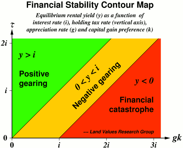
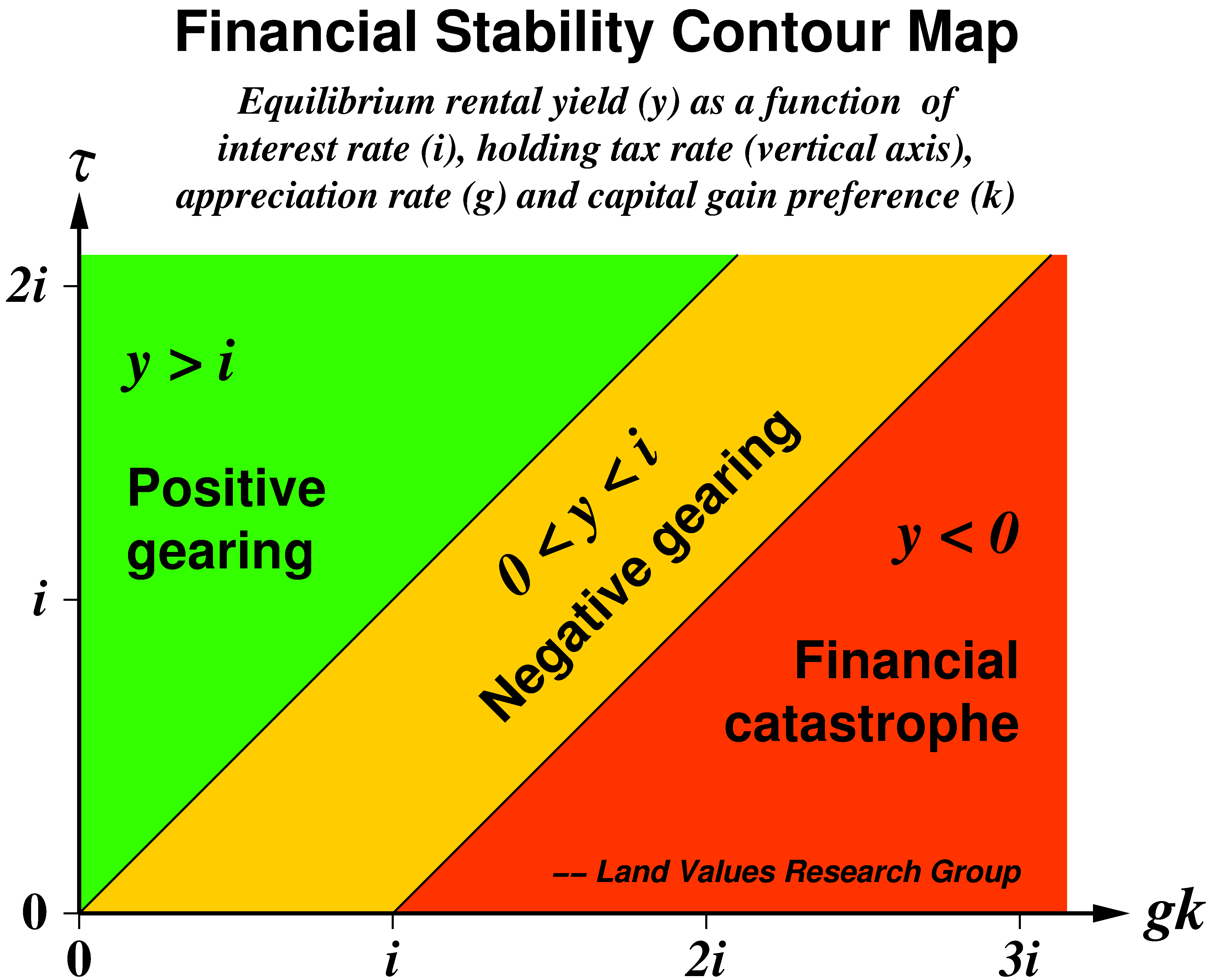
The financial stability contour map (above / hi-res version) shows how the tax system influences the property market so as to cause or prevent financial crises. It is a contour graph of the equilibrium rental yield (y) as a function of the holding tax rate (τ) and the product gk, where g is the appreciation rate (treated as exogenous) and k is the “capital-gain preference”, i.e. the factor by which the tax system magnifies capital gains relative to current income. The graph is calibrated in terms of the interest rate (i). If y falls to zero, “equilibrium” property prices become infinite. But obviously the financial system cannot support infinite prices. Hence, if the tax system is such that y is zero or negative, financial instability is guaranteed.

1.  The yield formula

Suppose that a property

• has a gross annual rental yield y,

• appreciates at an annual rate g (for “gain” or “growth”),

• can be mortgaged at an effective annual interest rate i, and

• is subject to a public holding charge or “land tax” at an annual rate τ,

where all four variables are expressed as decimals; e.g. if y=0.04, the yield is 4% per annum, and so on.

The “effective” interest rate is the interest paid on the debt-funded part of the purchase price plus the interest forgone on the remainder, all divided by the price.

In the case of an improved property (e.g. a property including a building), g is adjusted to account for depreciation/maintenance of the improvements, and τ, as defined here, is expressed in terms of the improved value (even if the rate defined by legislation is levied on the land value alone — as it should be, to avoid penalizing construction).

The applicable appreciation rate is that of a fixed address — not to be confused with that of the average property or the median property. As cities grow, average and median properties move further from city centres, so that their prices do not grow as fast as those of particular properties.

When the market reaches equilibrium — not in the sense that prices are constant, but rather in the sense that g is constant — buying must be competitive with renting. Hence the total return (that is, the rent saved or earned, plus the appreciation) must balance the total holding cost (the interest paid or forgone, plus the holding “tax”). On a per-unit-price basis, this is written

y + g = i + τ ,

(1)

whence

1/y = 1 / (i+τ-g) .

(2)

Of course 1/y is the P/E (price/earnings) ratio, which in practice must be positive, so that the denominator on the right-hand side must also be positive. As that denominator approaches zero, the P/E ratio “approaches infinity” — i.e. increases without limit.

In practice, of course, the P/E ratio must be finite, because borrowers have a limited capacity to service loans. Even if they plan to pay interest out of capital gains, the economy has a limited capacity to realize capital gains, which in turn limits borrowers' capacity to service loans. If that capacity is exceeded, there will be a financial crisis. Hence, if crisis is to be avoided, the P/E ratio set by the market must not exceed the capacity to service loans; that is, y must not be too low.

If the denominator on the right side of Eq.(2) is zero, any reduction in the interest rate or the holding charge or any increase in the appreciation rate will cause the denominator, hence the P/E ratio, to go negative. But any one of these changes should make one willing to pay more for the site, not less — as is clear if we substitute P/E  for 1/y and rearrange as follows:

P = (E+gP) / (i+τ) .

(3)

It is as if negative prices were not less than zero, but greater than infinity!

Not surprisingly, Eq.(3) indicates that if τ=0 (that is, if there is no “land tax” or other holding charge), the price is the annual accrual (rent plus capital gain) divided by the interest rate, and that the “land tax” affects the price like additional interest.

The latter conclusion could have been reached from Eq.(1): because interest and “land tax” appear as a sum, and only as a sum, “land tax” affects the price like additional interest. Of course it would be an equally valid interpretation to say that interest affects the price like another “land tax” — except that (a) interest is paid only by the lower class of property owners, namely those with mortgages, and (b) whereas a rise in the “land tax” rate requires legislative change and is regarded as politically impossible, a rise in interest rates requires nothing but the executive decision of a central bank that is not answerable to the voters.

Eq.(2) could have been derived from Eq.(3), which in turn can be derived by treating the price as the discounted present value of the future rent stream. In this approach, i is the discounting rate rather than the borrowing rate, and g is initially defined as the rate of increase in rent and is therefore exogenous (but this is still not enough to guarantee a finite price); details are given in the Appendix.

2.  Effect of taxes

If financial instability is to be avoided, the rental yield y as set by the market must be high enough (i.e., the P/E ratio must be low enough) to enable buyers to service loans. But the “market” is not oblivious to taxation.

Recurrent property taxes have already been taken into account (through τ).

A broad-based consumption tax, in so far as it simply devalues the currency in which all values are measured, has no effect on the above analysis. In theory, because “investment” in land delays the opportunity to consume, a consumption tax may affect land prices if it is known to discriminate between current and future consumption, whether because the tax rate will change or because the items that will be consumed later (after selling the land) will be taxed more or less severely than the items that could be consumed now (instead of buying the land). But in practice such effects are unlikely to be known or even guessed at, let alone acted upon. (The word “investment” is in quotation marks because “investment” in land does not of itself produce a new net asset.)

To account for income tax, all quantities in Eq.(1) — or all quantities except P in Eq.(3) — must be replaced by after-tax equivalents.

For convenience, let us define a neutral income tax as having a flat marginal rate, no discrimination between current income and capital gains, and full deductibility of interest and property taxes (that is, no quarantining of “negative gearing”). Under these conditions, the affected quantities are converted to their after-tax equivalents by multiplying by the scale factor (1-r), where r is the income-tax rate (e.g. r=0.3 for a 30% marginal rate). When this is done in Eq.(1) or (3), the factor (1-r) cancels out and the equation is left unchanged. So a neutral income tax does not affect P or the pre-tax P/E ratio.

The requirement that a “neutral” income tax has “no discrimination between current income and capital gains” does not apply to current income that is outside the present analysis, e.g. labour income. Discounting of income from assets relative to income from labour does not violate neutrality provided that rents, capital gains, interest and holding costs are all discounted by the same factor.

In Australia, the treatment of owner-occupied housing is an extreme case of uniform discounting: imputed rents and capital gains are not taxable, while interest and council rates are not deductible; so income tax is neutral. But for commercial and investment property, neutrality is violated in that capital gains alone are discounted for tax purposes. Hence, when we substitute after-tax equivalents in Eq.(1), the scale factor for g becomes (1-r′), where r′ is the effective rate of capital gains tax (CGT); and when we divide through by (1-r), the scale factors don't all cancel out, but g ends up being scaled by the factor

(1-r′)/(1-r) ,

which is greater than 1 (if capital gains are taxed less than current income). For brevity, let's call this factor k. So Eq.(1) gets modified as follows:

y + gk = i + τ .

(4)

For example, taxing capital gains at 15% and current income at 30% gives k=(1-0.15)/(1-0.3)=85/70. Exempting capital gains while taxing current income at 50% would give k=2. Taxing capital gains and current income at the same rate would give k=1. Taxing capital gains at 50% while exempting current income would give k=0.5. If k=0, capital gains are confiscated. In each case, it is assumed that interest and holding taxes are deductible at the same marginal tax rate at which rental income is taxable.

This simple scaling of the appreciation rate is valid for short-term or non-compounding appreciation. It does not work when compounding of appreciation is taken into account, as in the Appendix, because the tax advantage of capital gains does not compound. Thus, if the property is to be held for a long period, the applicable value of k is less extreme (i.e. closer to 1) than would be calculated from the tax rates. Indeed, according to the analysis in the Appendix, the condition for a finite price is that g<i. Because this condition does not involve k or τ, it implies that as the holding time becomes infinite, the effective value of k approaches 1, and neither the capital-gain discount nor the holding tax rate will make the difference between a finite price and an infinite price. But for a shorter holding time, either k or τ can make that difference; and even for an infinite holding time, either k or τ can make the difference between a sustainable equilibrium P/E ratio and an unsustainable one.

What about conveyancing stamp duty? From the viewpoint of someone who buys a property and re-sells it, the stamp duty is equivalent to a holding tax at a rate inversely proportional to the time for which the asset is held. In a rising market, it is alternatively equivalent to a capital gains tax at a rate inversely related to the time for which the asset is held. Either way, it tends to impose a lower limit on the holding time, but has little effect on buyers who intend to hold for long periods.

If the ability to deduct current losses on property against other income (“negative gearing”) is restricted in any way, the effect is equivalent to that of increasing the interest rate for the affected owners.

Because the present model is an equilibrium model, it doesn't predict the transient effects of changes in the tax system. For example, there is empirical evidence that a new stamp-duty concession (or a new grant!) for a particular class of buyers will bring forward demand from that class, and that the counterparties will “lever up” their capital gains through the financial system in order to “trade up”, and so on, causing a temporary speculative spiral. The aim of the present model is not to predict those dynamics, but rather to determine whether the tax system is compatible with financial stability. As the word “stability” suggests, an equilibrium model is satisfactory for that purpose.

3.  Note on inflation

In the above analysis, capital gains and interest have been taken as nominal. This is appropriate for Australia, where the tax system assesses nominal capital gains and allows deductions for nominal interest. If the tax system assessed real capital gains (all else being unchanged), that would be represented by a higher value of k. If only real interest were deductible (all else being unchanged), the effect would be equivalent to that of a higher interest rate.

4.  The contour graph

Eq.(4) can be written in the form

gk = τ + i-y ,

(5)

which shows that the graph of gk vs. τ is a straight line, with unit slope and an intercept of i-y on the “gk axis”. Each value of y gives a different line, so that each line can be understood as a contour in a graph of y vs. gk and τ. Because the intercept (i-y) is a linear function of y, equally spaced values of y give equally spaced contours.

The most interesting contours are y=0, for which the intercept is i, and y=i, for which the intercept is 0. From these we may deduce the regions for which y>i (positive gearing at 100% LVR), 0<y<i (negative gearing), and y<0 (guaranteed financial instability), as shown in the graph above (reproduced below).

Because equally spaced values of y give equally spaced contours, we can easily add contours for other values of y. For example, the contour for y=i/2, for which the equilibrium rental yield is half the interest rate, is in the middle of the “negative gearing” band. Empirically, a rental yield of less than half the interest rate should make one fear an imminent crash. Hence, if the tax system is such that y<i/2 — that is, if it places us closer to the red region of the contour map than the green region — it invites a strong suspicion that the tax system is incompatible with long-term financial stability. If the tax system places us in the red region, suspicion gives way to certainty.

If the tax system causes the “equilibrium” rental yield to be unsustainably low, prices will rise until the financial system collapses, then fall until the bad debts are somehow worked out, then rise again, and so on. At any stage of the cycle, the price of a property will be determined by what one can borrow against it.

5.  Where are we?

In Australia, the long-term appreciation rate is similar to the long-term interest rate. For residential owner-occupants, k=1, so gk is roughly i; and the property tax rate is a small fraction of i. That places us close to the red region — too close for financial stability. For other classes of property owners, k is higher, and the total property tax rate is also higher, but probably by an insufficient margin to compensate for the higher k, in which case the destabilizing tendency is even greater than that from ordinary home owners.

Under these conditions, arguments about population growth and the unresponsiveness of housing supply are relevant to the direction of rents, but not to the direction of prices or price/rent ratios, which are limited by the financial system.

6.  Implications

If the tax system places us in the red region, raising interest rates might shift us into the amber region. But because monetary policy affects prices of goods and services, it is not necessarily available for the purpose of taming asset prices. Moreover, the above analysis deals with constant interest rates, not changes in interest rates. In reality, of course, if high property prices have endangered the financial system, raising interest rates will tend to precipitate the collapse.

As explained in the preceding article in this series, financial regulations aimed at limiting credit on the supply side are not politically robust.

So we must look to the tax system. In the long term, financial stability is improved by higher “land tax” and/or higher taxation of capital gains relative to current income (including at least income from assets). At present, capital gains are taxed less than income from assets. If it were the other way around, financial crises would be less likely. Any of these reforms, by making it more attractive to generate income from land and less attractive to hold idle land in pursuit of capital gains, would improve the responsiveness of housing supply to population growth, reducing g and improving financial stability. Any of these reforms involves a change in the tax mix. None of them requires an overall increase in taxation.

Implications for housing affordability are considered in the next post.

Appendix.  Present value of future rent

The sum

S = A + AR + AR² + AR³ + AR⁴ + ...

(6)

is called an infinite geometric series in which A is the first term and R is the common ratio (the ratio of each subsequent term to its predecessor).

If |R| is greater than 1, obviously the sum is infinite; it just keeps getting bigger as we keep adding terms. If |R| is equal to 1, successive terms don't get smaller, so the sum can't “settle down”.

But what if |R| is less than 1? First note that removing the first term is equivalent to multiplying each term, and hence the whole sum, by R; that is,

S - A = RS .

(7)

Then to remove the second term is to multiply the remaining sum by R, and so on. Then notice that because |R|<1, multiplying the sum by R means shrinking it, so that each successive removal shrinks the remaining sum by the same ratio. In other words, if we add the terms from left to right, each successive addition takes us closer to the sum S by the same ratio, which means that although there are infinitely many terms, the sum S is finite. To find that sum, we solve Eq.(7) for S, obtaining

S = A / (1-R) .

(8)

We can use this formula to find the P/E ratio. In the first year the property will yield yP in rent and be liable for τP in “tax”, giving a net positive cash flow of (y-τ)P. If this cash flow occurs at the end of the year, its present value (discounted by one year at the interest rate i) is

A = (y-τ)P / (1+i) .

(9)

Let us now assume that the rental value appreciates at a constant rate (g). At equilibrium (if that is possible), we have a constant yield, so that the price appreciates at the same rate. At equilibrium we also have constant i and τ, so that all related cash flows appreciate at the same rate. In each subsequent year, the net cash flow increases by a factor (1+g) and is discounted by a further factor (1+i). So the price P is an infinite geometric series whose first term is given by Eq.(9) and whose common ratio is

R = (1+g) / (1+i) .

(10)

If g<i, this ratio will be smaller than 1, so that we can use Eq.(8): substituting Eqs.(9) and (10) into Eq.(8), renaming S as P, renaming y as E/P, and simplifying, we get Eq.(3) again.

__________

^∗ First posted Nov.16, 2011; last modified Dec.23.